
Four Ways to Flag an Anomaly: What Runs Inside Grayson TimeSeries
Compare Z-score, IQR, Isolation Forest, and VAE anomaly detection methods: assumptions, strengths, limitations, and how Grayson TimeSeries uses them.
In this article
An anomaly is not always a reading that crosses a fixed limit. It can also be a value, pattern, or combination of variables that does not fit how the process normally behaves.
The problem is that every anomaly detection method defines “normal” differently. Z-score looks at distance from the mean. IQR looks at the middle of the distribution. Isolation Forest looks for observations that are easier to separate from the rest of the data. A variational autoencoder learns the underlying structure of normal operating data and looks for observations that do not fit it.
If the method’s assumptions do not match the dataset, an engineer can miss the excursion or spend the shift clearing false positives. That is why Grayson TimeSeries supports four anomaly detection methods and can run one or several against the same dataset. The engineer can compare the results and decide which method best fits the process and the question being investigated.
| Method | What it treats as unusual | Best fit | Main limitation |
|---|---|---|---|
| Z-score | Distance from a stable mean | Transparent, univariate screening | Sensitive to skew, drift, and changing operating regimes |
| IQR | Values beyond quartile-based fences | Skewed, univariate signals | Does not capture relationships between variables |
| Isolation Forest | Observations isolated in fewer random partitions | Unusual multivariable combinations | Less directly interpretable |
| Variational autoencoder | Data reconstructed poorly from learned normal structure | Contextual and non-linear patterns | Needs more history and compute; least directly interpretable |
Z-score: a transparent statistical baseline
Z-score measures how many standard deviations a reading sits above or below the mean. A reading with a Z-score of 3, for example, is three standard deviations away from the mean of the data being analyzed.
Its advantage is transparency. It is computationally light, easy to explain, and straightforward to audit. If Grayson flags a tag at 3σ, an engineer can reproduce the calculation by hand or check it in Excel.
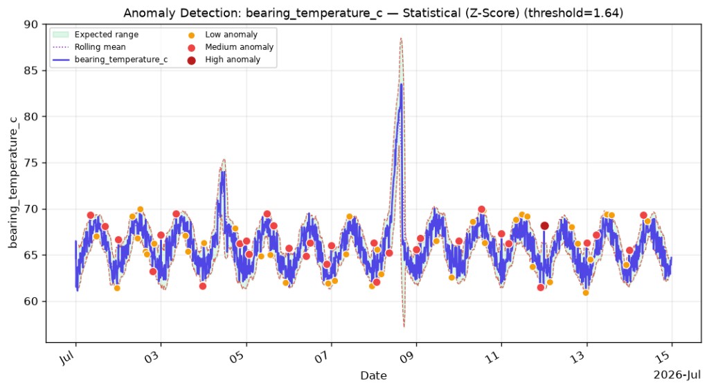
Z-score works best when the data is approximately normally distributed and the mean and variance remain reasonably stable. It becomes less reliable with heavily skewed signals, multiple operating regimes, or changing process conditions. If the baseline is continuously recalculated, a slow degradation trend can also pull the mean along with it and make the developing problem appear normal.
IQR: more resistant to skew and extreme values
Interquartile range uses the middle 50 percent of the data rather than the mean and standard deviation. It calculates the distance between the first quartile (Q1) and third quartile (Q3), then flags values falling below Q1 − 1.5×IQR or above Q3 + 1.5×IQR.
Because it is based on quartiles, the method is not heavily distorted by the extreme values it is trying to find. This makes IQR useful for skewed process variables where a handful of high or low readings could distort the mean.
The limitation is that IQR is normally applied one variable at a time. It can flag a drop in lube oil pressure, but it does not identify that the pressure drop preceded a rise in trunnion oil temperature. Each reading may be unusual on its own, but the relationship between the two variables is outside what IQR is designed to detect.
Isolation Forest: finding unusual combinations
Isolation Forest approaches the problem differently. Instead of defining a statistical boundary around normal data, it repeatedly selects a feature and splits the data at random. Observations in sparse or unusual parts of the feature space tend to be isolated in fewer splits, so shorter path lengths produce higher anomaly scores.
It does not require the data to follow a normal distribution and can analyze multiple variables together. This makes it useful when the individual readings appear reasonable but their combination is unusual.
Motor current may be within range. Vibration may also be within range. But that particular combination of motor current and vibration may be unusual at the recorded feed rate. Isolation Forest can identify that relationship even when none of the individual variables crosses a fixed threshold.
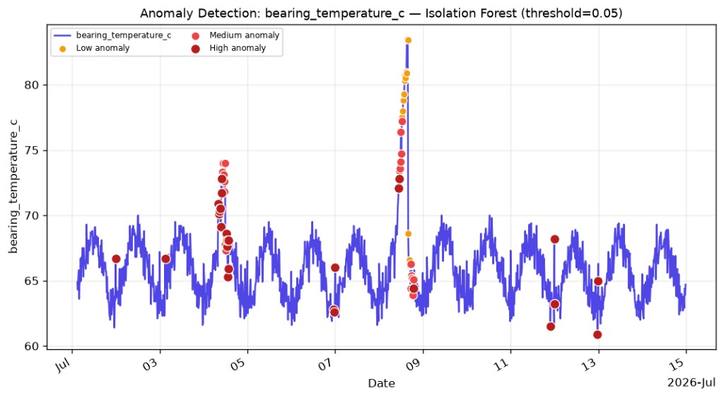
The tradeoff is interpretability. Its result is not as easy to check by hand as a Z-score or an IQR boundary, and the variables, operating regimes, and data window included in the analysis can materially affect the result.
Variational autoencoder: detecting values that are wrong for the operating state
A variational autoencoder, or VAE, learns a compressed representation of normal operating data and then attempts to reconstruct it. When new data does not match the structure the model learned, the reconstruction error increases and the observation can be flagged for investigation. Reconstruction error is one established way to use VAEs for anomaly detection, although the threshold still needs to be calibrated for the application.
This is useful for contextual anomalies. A reading may fall within its normal operating limits but still be wrong for what the process is doing at that moment. Values associated with steady-state operation, for example, may be individually reasonable but unusual if they appear halfway through startup.
A VAE can capture more complex, non-linear relationships across several variables, but it generally needs more operating history and more computation than the simpler statistical methods. It is also the least directly interpretable of the four, which makes comparison with the other methods and a clear audit trail particularly important.
Why run more than one anomaly detection method?
There is no universal winner across industrial datasets. Z-score and IQR are fast, transparent, and often sufficient for straightforward tag-level screening. Isolation Forest and VAE can detect multivariable or contextual behaviour that simpler statistical boundaries may miss.
Running several methods does not mean treating every flag as a process fault. It gives the engineer several definitions of normal to compare. If multiple methods flag the same period, that strengthens the case for investigation. If they disagree, the disagreement itself can reveal something about the distribution, operating state, or relationships inside the data.
The point is not to throw more algorithms at the dataset for the sake of it. It is to avoid staking an operational conclusion on one model’s assumptions before seeing whether those assumptions actually fit the process.
Grayson TimeSeries lets engineers run one or multiple anomaly detection methods from Microsoft Teams, compare the results, review the visualization, and download an audit trail showing what data, algorithms, and parameters were used.
Upload an Excel or CSV export, ask the question in plain language, and see which definition of “normal” best explains what is happening in your process.
Add Grayson TimeSeries to Microsoft Teams and run your first anomaly analysis.
Technical references
Grayson TimeSeries: supported analyses and anomaly detection methods
NIST Engineering Statistics Handbook: Z-scores and standardization
NIST Engineering Statistics Handbook: quartiles and interquartile range
Liu, Ting, and Zhou: “Isolation Forest”
Kingma and Welling: “Auto-Encoding Variational Bayes”
Škvára et al.: “Anomaly Detection with Variational Autoencoders”
Next step
Install, run a first analysis, or keep reading
Support covers setup in Microsoft Teams. The Knowledge Hub collects the worked examples and industry notes.